Wave Energy
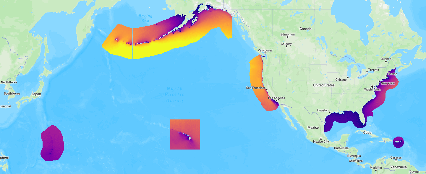
Ocean waves have an estimated 1,400 TWh/yr of technical energy potential across the U.S. EEZ, equivalent to 34% of U.S. electricity generation [@general_kilcher2021_marine]. The U.S. Department of Energy's Hydropower and Hydrokinetic Office (H2O) produced a 42-year, high-resolution hindcast covering all U.S. coastal and offshore waters to map that resource in detail. The data are freely accessible through the Marine Energy Atlas, a Python API, and raw HDF5 files on AWS S3.
What Is a Hindcast?
A hindcast is a numerical model simulation that estimates past wave conditions over a defined area and time period using historical forcing and boundary conditions. It reconstructs how conditions varied over time and space across a much larger area than can be captured by real-world measurements alone. Hindcasts are particularly valuable for marine energy resource characterization because measured data are often very sparse in both time and location; without a hindcast, the available observations may be too limited to fully describe the resource or operating conditions at a site. By providing a spatially and temporally continuous record, hindcasts help fill those gaps and support resource assessment, site screening, engineering design, and evaluation of long-term variability.
Regional Datasets
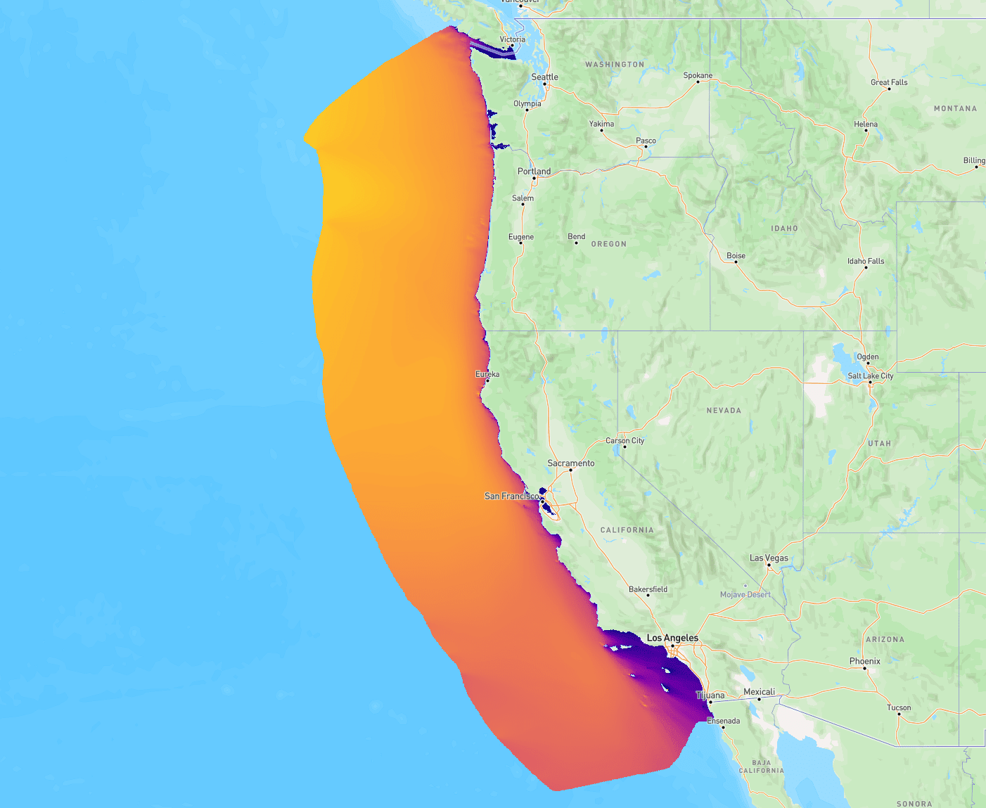
West Coast
[chicago@wu2020_west_coast]
- Period: 1979–2020 · 42 annual files
- Total archive: ~3.3 TB
- Version:
v1.0.1
2011–2020 (10 files)
- Grid points: 699,904 · ~71.7 GB per year
Variable definitions (9) · 2011–2020
| Variable | Description | IEC Name | SWAN name | Units |
|---|---|---|---|---|
directionality_coefficient |
Directionality coefficient | \(d\) | ||
energy_period |
Energy period | \(T_{e}\), \(T_{-10}\) | TMM10 | s |
maximum_energy_direction |
Peak wave direction (nautical convention) | PDIR | degr | |
mean_absolute_period |
Mean absolute wave period - equivalent to T_m01 | PER | s | |
mean_wave_direction |
Mean wave direction (nautical convention) | DIR | degr | |
omni-directional_wave_power |
Omnidirectional wave power | \(J\) | W/m | |
peak_period |
Relative peak period of the variance density spectrum | \(T_{p}\) | RTP | s |
significant_wave_height |
Significant wave height | \(H_{m0}\) | HSIGN | m |
spectral_width |
Spectral width | \(\epsilon_{0}\) |
Variable schema (9) · 2011–2020
| Variable | Units | Dimensions | Type |
|---|---|---|---|
directionality_coefficient |
2,928 × 699,904 | float32 |
|
energy_period |
s | 2,928 × 699,904 | float32 |
maximum_energy_direction |
degr | 2,928 × 699,904 | float32 |
mean_absolute_period |
s | 2,928 × 699,904 | float32 |
mean_wave_direction |
degr | 2,928 × 699,904 | float32 |
omni-directional_wave_power |
W/m | 2,928 × 699,904 | float32 |
peak_period |
s | 2,928 × 699,904 | float32 |
significant_wave_height |
m | 2,928 × 699,904 | float32 |
spectral_width |
2,928 × 699,904 | float32 |
Metadata (6 fields) · 2011–2020
| Field | Type |
|---|---|
water_depth |
float32 |
latitude |
float32 |
longitude |
float32 |
distance_to_shore |
float32 |
timezone |
int16 |
jurisdiction |
str[20] |
1979–2010 (32 files)
- Grid points: 699,904 · ~81.9 GB per year
Variable definitions (10) · 1979–2010
| Variable | Description | IEC Name | SWAN name | Units |
|---|---|---|---|---|
directionality_coefficient |
Directionality coefficient | \(d\) | ||
energy_period |
Energy period | \(T_{e}\), \(T_{-10}\) | TMM10 | s |
maximum_energy_direction |
Direction of maximum directionally resolved wave power (nautical convention) | \(\theta_{J}\) | degr | |
mean_absolute_period |
Mean absolute wave period - equivalent to T_m01 | PER | s | |
mean_wave_direction |
Mean wave direction (nautical convention) | DIR | degr | |
mean_zero-crossing_period |
Mean absolute zero-crossing period | \(T_{z}\), \(T_{02}\) | TM02 | s |
omni-directional_wave_power |
Omnidirectional wave power | \(J\) | W/m | |
peak_period |
Relative peak period of the variance density spectrum | \(T_{p}\) | RTP | s |
significant_wave_height |
Significant wave height | \(H_{m0}\) | HSIGN | m |
spectral_width |
Spectral width | \(\epsilon_{0}\) |
Variable schema (10) · 1979–2010
| Variable | Units | Dimensions | Type |
|---|---|---|---|
directionality_coefficient |
2,920 × 699,904 | float32 |
|
energy_period |
s | 2,920 × 699,904 | float32 |
maximum_energy_direction |
degr | 2,920 × 699,904 | float32 |
mean_absolute_period |
s | 2,920 × 699,904 | float32 |
mean_wave_direction |
degr | 2,920 × 699,904 | float32 |
mean_zero-crossing_period |
s | 2,920 × 699,904 | float32 |
omni-directional_wave_power |
W/m | 2,920 × 699,904 | float32 |
peak_period |
s | 2,920 × 699,904 | float32 |
significant_wave_height |
m | 2,920 × 699,904 | float32 |
spectral_width |
2,920 × 699,904 | float32 |
Metadata (6 fields) · 1979–2010
| Field | Type |
|---|---|
water_depth |
float32 |
latitude |
float32 |
longitude |
float32 |
distance_to_shore |
float32 |
timezone |
int16 |
jurisdiction |
str[20] |
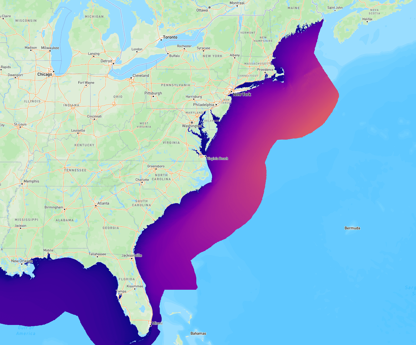
East Coast
[chicago@ahn2021_east_coast]
- Period: 1979–2020 · 42 annual files
- Total archive: ~12.7 TB
- Version:
v1.0.1
2011–2020 (10 files)
- Grid points: 2,635,135 · ~316.2 GB per year
Variable definitions (11) · 2011–2020
| Variable | Description | IEC Name | SWAN name | Units |
|---|---|---|---|---|
directionality_coefficient |
Directionality coefficient | \(d\) | ||
energy_period |
Energy period | \(T_{e}\), \(T_{-10}\) | TMM10 | s |
maximum_energy_direction |
Direction of maximum directionally resolved wave power (nautical convention) | \(\theta_{J}\) | deg | |
mean_absolute_period |
Mean absolute wave period - equivalent to T_m01 | PER | s | |
mean_wave_direction |
Mean wave direction (nautical convention) | DIR | deg | |
mean_zero-crossing_period |
Mean absolute zero-crossing period | \(T_{z}\), \(T_{02}\) | TM02 | s |
omni-directional_wave_power |
Omnidirectional wave power | \(J\) | W/m | |
peak_period |
Relative peak period of the variance density spectrum | \(T_{p}\) | RTP | s |
peak_period_direction |
Peak wave direction (nautical convention) | PDIR | deg | |
significant_wave_height |
Significant wave height | \(H_{m0}\) | HSIGN | m |
spectral_width |
Spectral width | \(\epsilon_{0}\) |
Variable schema (11) · 2011–2020
| Variable | Units | Dimensions | Type |
|---|---|---|---|
directionality_coefficient |
2,928 × 2,635,135 | float32 |
|
energy_period |
s | 2,928 × 2,635,135 | float32 |
maximum_energy_direction |
deg | 2,928 × 2,635,135 | float32 |
mean_absolute_period |
s | 2,928 × 2,635,135 | float32 |
mean_wave_direction |
deg | 2,928 × 2,635,135 | float32 |
mean_zero-crossing_period |
s | 2,928 × 2,635,135 | float32 |
omni-directional_wave_power |
W/m | 2,928 × 2,635,135 | float32 |
peak_period |
s | 2,928 × 2,635,135 | float32 |
peak_period_direction |
deg | 2,928 × 2,635,135 | float32 |
significant_wave_height |
m | 2,928 × 2,635,135 | float32 |
spectral_width |
2,928 × 2,635,135 | float32 |
1979–2010 (32 files)
- Grid points: 2,635,135 · ~308.1 GB per year
Variable definitions (10) · 1979–2010
| Variable | Description | IEC Name | SWAN name | Units |
|---|---|---|---|---|
directionality_coefficient |
Directionality coefficient | \(d\) | ||
energy_period |
Energy period | \(T_{e}\), \(T_{-10}\) | TMM10 | s |
maximum_energy_direction |
Direction of maximum directionally resolved wave power (nautical convention) | \(\theta_{J}\) | deg | |
mean_absolute_period |
Mean absolute wave period - equivalent to T_m01 | PER | s | |
mean_wave_direction |
Mean wave direction (nautical convention) | DIR | deg | |
mean_zero-crossing_period |
Mean absolute zero-crossing period | \(T_{z}\), \(T_{02}\) | TM02 | s |
omni-directional_wave_power |
Omnidirectional wave power | \(J\) | W/m | |
peak_period |
Relative peak period of the variance density spectrum | \(T_{p}\) | RTP | s |
significant_wave_height |
Significant wave height | \(H_{m0}\) | HSIGN | m |
spectral_width |
Spectral width | \(\epsilon_{0}\) |
Variable schema (10) · 1979–2010
| Variable | Units | Dimensions | Type |
|---|---|---|---|
directionality_coefficient |
2,920 × 2,635,135 | float32 |
|
energy_period |
s | 2,920 × 2,635,135 | float32 |
maximum_energy_direction |
deg | 2,920 × 2,635,135 | float32 |
mean_absolute_period |
s | 2,920 × 2,635,135 | float32 |
mean_wave_direction |
deg | 2,920 × 2,635,135 | float32 |
mean_zero-crossing_period |
s | 2,920 × 2,635,135 | float32 |
omni-directional_wave_power |
W/m | 2,920 × 2,635,135 | float32 |
peak_period |
s | 2,920 × 2,635,135 | float32 |
significant_wave_height |
m | 2,920 × 2,635,135 | float32 |
spectral_width |
2,920 × 2,635,135 | float32 |
Metadata (6 fields) · 1979–2010
| Field | Type |
|---|---|
latitude |
float32 |
longitude |
float32 |
water_depth |
float32 |
timezone |
int16 |
distance |
float32 |
jurisdiction |
str[14] |
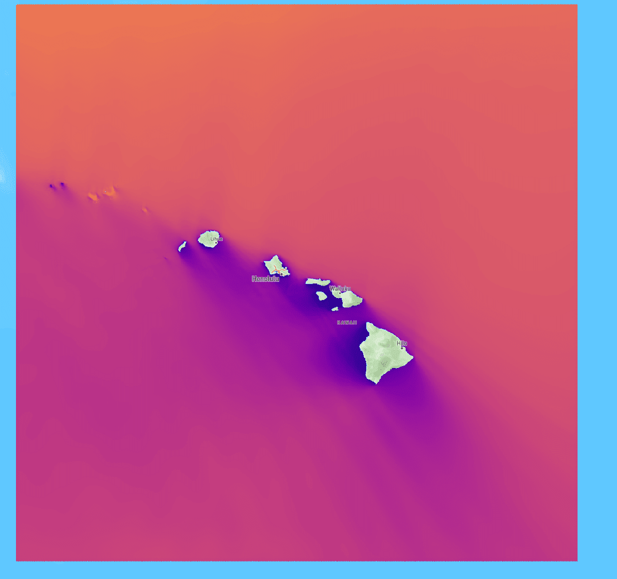
Hawaii
[chicago@li2021_hawaii]
Covers the full Hawaiian Archipelago EEZ, including every island and atoll in both the Northwestern Hawaiian Islands (Marine National Monument) and the Main Hawaiian Islands:
- State of Hawaii
- Niihau
- Kauai
- Oahu
- Molokai
- Lanai
- Kahoolawe
- Maui
- Hawaii (Big Island)
- Northwestern Hawaiian Islands
- Kure Atoll
- Midway Atoll
- Pearl and Hermes Atoll
- Lisianski Island
- Laysan Island
- Maro Reef
- Gardner Pinnacles
- French Frigate Shoals
- Necker Island
- Nihoa
- Period: 1979–2020 · 42 annual files
- Total archive: ~4.4 TB
- Version:
v1.0.0
2011–2020 (10 files)
- Grid points: 1,696,188 · ~189.7 GB per year
Variable definitions (10) · 2011–2020
| Variable | Description | IEC Name | SWAN name | Units |
|---|---|---|---|---|
depth |
Water depth | Depth | m | |
directionality_coefficient |
Directionality coefficient | \(d\) | ||
energy_period |
Energy period | \(T_{e}\), \(T_{-10}\) | TMM10 | s |
maximum_energy_direction |
Peak wave direction (nautical convention) | PDIR | degr | |
mean_absolute_period |
Mean absolute wave period - equivalent to T_m01 | PER | s | |
mean_wave_direction |
Mean wave direction (nautical convention) | DIR | degr | |
omni-directional_wave_power |
Omnidirectional wave power | \(J\) | W/m | |
peak_period |
Relative peak period of the variance density spectrum | \(T_{p}\) | RTP | s |
significant_wave_height |
Significant wave height | \(H_{m0}\) | HSIGN | m |
spectral_width |
Spectral width | \(\epsilon_{0}\) |
Variable schema (10) · 2011–2020
| Variable | Units | Dimensions | Type |
|---|---|---|---|
depth |
m | 2,928 × 1,696,188 | float32 |
directionality_coefficient |
2,928 × 1,696,188 | float32 |
|
energy_period |
s | 2,928 × 1,696,188 | float32 |
maximum_energy_direction |
degr | 2,928 × 1,696,188 | float32 |
mean_absolute_period |
s | 2,928 × 1,696,188 | float32 |
mean_wave_direction |
degr | 2,928 × 1,696,188 | float32 |
omni-directional_wave_power |
W/m | 2,928 × 1,696,188 | float32 |
peak_period |
s | 2,928 × 1,696,188 | float32 |
significant_wave_height |
m | 2,928 × 1,696,188 | float32 |
spectral_width |
2,928 × 1,696,188 | float32 |
Metadata (7 fields) · 2011–2020
| Field | Type |
|---|---|
latitude |
float32 |
longitude |
float32 |
depth |
float32 |
distance_to_shore |
float32 |
timezone |
int16 |
eez |
str[13] |
jurisdiction |
str[14] |
1979–2010 (32 files)
- Grid points: 700,414 · ~81.9 GB per year
Variable definitions (10) · 1979–2010
| Variable | Description | IEC Name | SWAN name | Units |
|---|---|---|---|---|
directionality_coefficient |
Fraction of total wave energy travelling in the "direction of maximum wave power" direction | \(d\) | ||
energy_period |
Spectral width characterizes the relative spreading of energy in the wave spectrum. Large values indicate a wider spectral peak | \(T_{e}\) | TM02 | s |
maximum_energy |
Maximum directionally resolved wave energy | \(J_{\sigma,jdmax}\) | jdmax | W/m |
maximum_energy_direction |
The direction from which the most wave energy is travelling | \(Jsigma_{Jmax}\) | deg | |
mean_absolute_period |
Resolved Spectral Moment (m_0/m_1) | \(T_{p}\) | PER | s |
mean_wave_direction |
Direction Normal to the Wave Crests | \(\Sigma\) | DIR | deg |
omni-directional_wave_power |
Total wave energy flux from all directions | \(J\) | W/m | |
peak_period |
The period associated with the maximum value of the wave energy spectrum | \(T_{p}\) | RTP | s |
significant_wave_height |
Calculated as the zeroth spectral moment (i.e., H_m0) | \(H_{s}\) | HSIGN | m |
spectral_width |
Spectral width characterizes the relative spreading of energy in the wave spectrum. Large values indicate a wider spectral peak | \(\epsilon_{0}\) |
Variable schema (10) · 1979–2010
| Variable | Units | Dimensions | Type |
|---|---|---|---|
directionality_coefficient |
2,920 × 700,414 | float32 |
|
energy_period |
s | 2,920 × 700,414 | float32 |
maximum_energy |
W/m | 2,920 × 700,414 | float32 |
maximum_energy_direction |
deg | 2,920 × 700,414 | float32 |
mean_absolute_period |
s | 2,920 × 700,414 | float32 |
mean_wave_direction |
deg | 2,920 × 700,414 | float32 |
omni-directional_wave_power |
W/m | 2,920 × 700,414 | float32 |
peak_period |
s | 2,920 × 700,414 | float32 |
significant_wave_height |
m | 2,920 × 700,414 | float32 |
spectral_width |
2,920 × 700,414 | float32 |
Metadata (6 fields) · 1979–2010
| Field | Type |
|---|---|
latitude |
float32 |
longitude |
float32 |
distance_to_shore |
float32 |
timezone |
int16 |
jurisdiction |
str[7] |
water_depth |
float32 |
Alaska
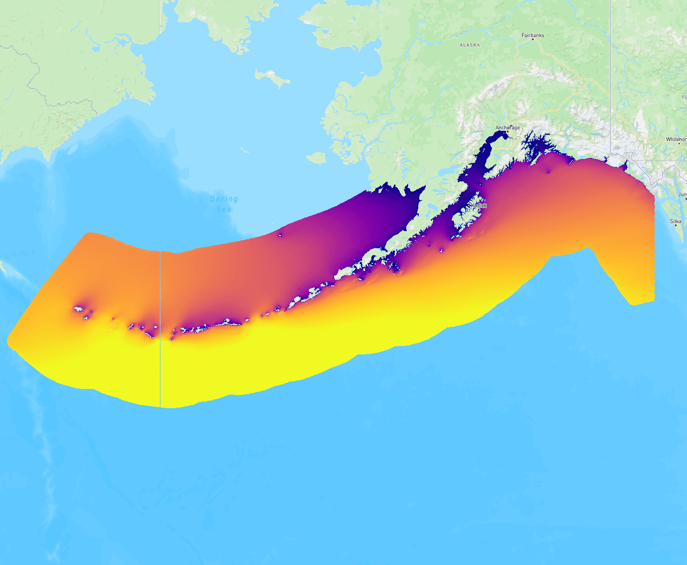
[chicago@garcia_medina2021_us_alaska]
- Period: 1979–2020 · 42 annual files
- Total archive: ~18.1 TB
- Version:
v1.0.1
2011–2020 (10 files)
- Grid points: 3,894,283 · ~399.1 GB per year
Variable definitions (9) · 2011–2020
| Variable | Description | IEC Name | SWAN name | Units |
|---|---|---|---|---|
directionality_coefficient |
Directionality coefficient | \(d\) | ||
energy_period |
Energy period | \(T_{e}\), \(T_{-10}\) | TMM10 | s |
maximum_energy_direction |
Direction of maximum directionally resolved wave power (nautical convention) | \(\theta_{J}\) | degr | |
mean_absolute_period |
Mean absolute wave period - equivalent to T_m01 | PER | s | |
mean_wave_direction |
Mean wave direction (nautical convention) | DIR | degr | |
omni-directional_wave_power |
Omnidirectional wave power | \(J\) | W/m | |
peak_period |
Relative peak period of the variance density spectrum | \(T_{p}\) | RTP | s |
significant_wave_height |
Significant wave height | \(H_{m0}\) | HSIGN | m |
spectral_width |
Spectral width | \(\epsilon_{0}\) |
Variable schema (9) · 2011–2020
| Variable | Units | Dimensions | Type |
|---|---|---|---|
directionality_coefficient |
2,928 × 3,894,283 | float32 |
|
energy_period |
s | 2,928 × 3,894,283 | float32 |
maximum_energy_direction |
degr | 2,928 × 3,894,283 | float32 |
mean_absolute_period |
s | 2,928 × 3,894,283 | float32 |
mean_wave_direction |
degr | 2,928 × 3,894,283 | float32 |
omni-directional_wave_power |
W/m | 2,928 × 3,894,283 | float32 |
peak_period |
s | 2,928 × 3,894,283 | float32 |
significant_wave_height |
m | 2,928 × 3,894,283 | float32 |
spectral_width |
2,928 × 3,894,283 | float32 |
Metadata (6 fields) · 2011–2020
| Field | Type |
|---|---|
latitude |
float32 |
longitude |
float32 |
timezone |
float32 |
distance |
float32 |
jurisdiction |
str[7] |
water_depth |
float32 |
1979–2010 (32 files)
- Grid points: 3,894,283 · ~455.2 GB per year
Variable definitions (10) · 1979–2010
| Variable | Description | IEC Name | SWAN name | Units |
|---|---|---|---|---|
directionality_coefficient |
Directionality coefficient | \(d\) | ||
energy_period |
Energy period | \(T_{e}\), \(T_{-10}\) | TMM10 | s |
maximum_energy_direction |
Direction of maximum directionally resolved wave power (nautical convention) | \(\theta_{J}\) | degr | |
mean_absolute_period |
Mean absolute wave period - equivalent to T_m01 | PER | s | |
mean_wave_direction |
Mean wave direction (nautical convention) | DIR | degr | |
mean_zero-crossing_period |
Mean absolute zero-crossing period | \(T_{z}\), \(T_{02}\) | TM02 | s |
omni-directional_wave_power |
Omnidirectional wave power | \(J\) | W/m | |
peak_period |
Relative peak period of the variance density spectrum | \(T_{p}\) | RTP | s |
significant_wave_height |
Significant wave height | \(H_{m0}\) | HSIGN | m |
spectral_width |
Spectral width | \(\epsilon_{0}\) |
Variable schema (10) · 1979–2010
| Variable | Units | Dimensions | Type |
|---|---|---|---|
directionality_coefficient |
2,920 × 3,894,283 | float32 |
|
energy_period |
s | 2,920 × 3,894,283 | float32 |
maximum_energy_direction |
degr | 2,920 × 3,894,283 | float32 |
mean_absolute_period |
s | 2,920 × 3,894,283 | float32 |
mean_wave_direction |
degr | 2,920 × 3,894,283 | float32 |
mean_zero-crossing_period |
s | 2,920 × 3,894,283 | float32 |
omni-directional_wave_power |
W/m | 2,920 × 3,894,283 | float32 |
peak_period |
s | 2,920 × 3,894,283 | float32 |
significant_wave_height |
m | 2,920 × 3,894,283 | float32 |
spectral_width |
2,920 × 3,894,283 | float32 |
Metadata (6 fields) · 1979–2010
| Field | Type |
|---|---|
latitude |
float32 |
longitude |
float32 |
timezone |
float32 |
distance |
float32 |
jurisdiction |
str[7] |
water_depth |
float32 |
Guam and Northern Mariana Islands
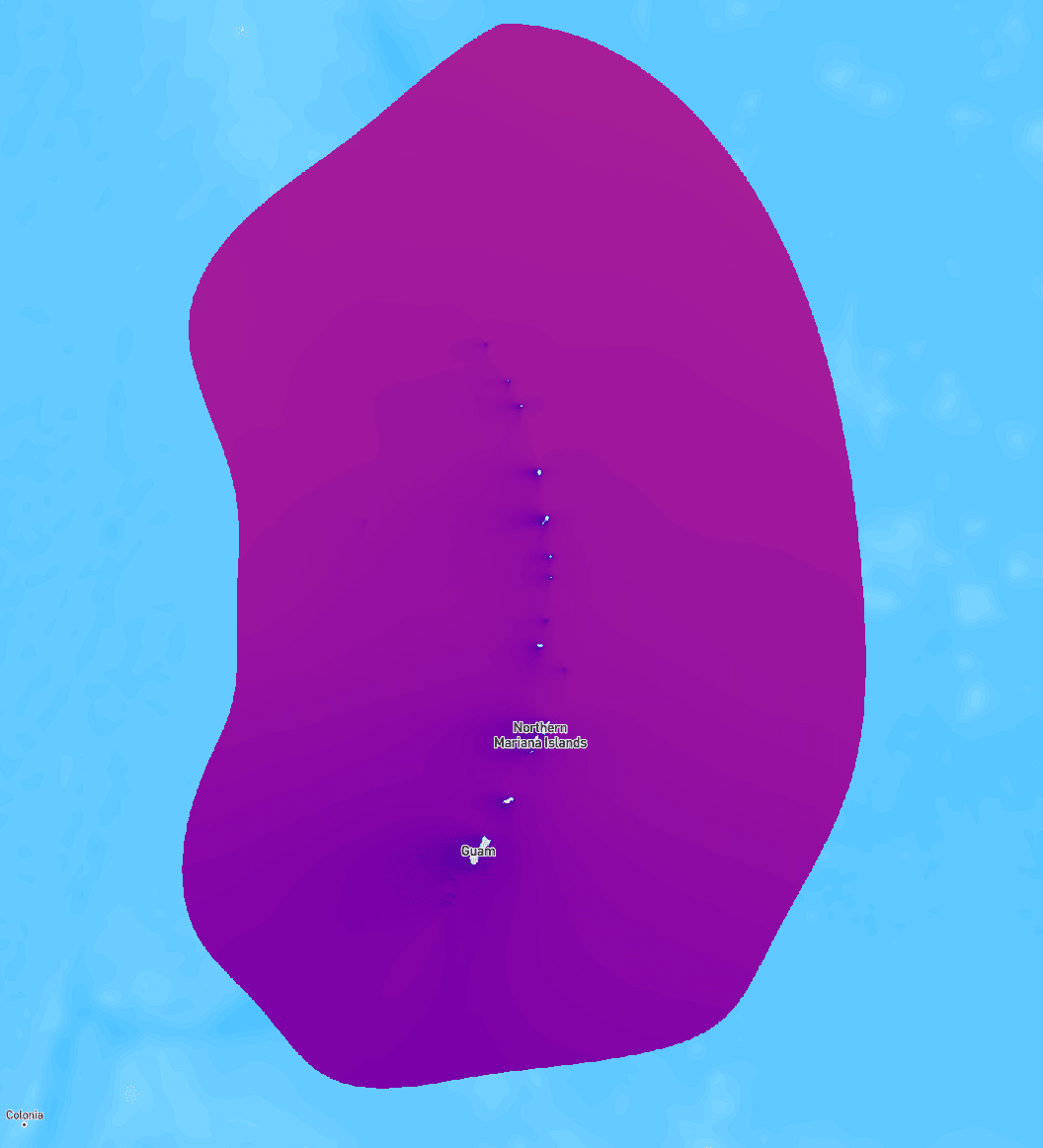
[chicago@garcia_medina2023_us_guam_and_cnmi]
- Grid points: 461,465
- File size: ~47.3 GB per year
- Period: 1979–2020 · 42 annual files
- Total archive: ~1.9 TB
- Version:
v1.0.0
Variable definitions (9)
| Variable | Description | IEC Name | SWAN name | Units |
|---|---|---|---|---|
directionality_coefficient |
Directionality coefficient | \(d\) | ||
energy_period |
Energy period | \(T_{e}\), \(T_{-10}\) | TMM10 | s |
maximum_energy_direction |
Direction of maximum directionally resolved wave power (nautical convention) | \(\theta_{J}\) | degr | |
mean_absolute_period |
Mean absolute wave period - equivalent to T_m01 | PER | s | |
mean_wave_direction |
Mean wave direction (nautical convention) | DIR | degr | |
omni-directional_wave_power |
Omnidirectional wave power | \(J\) | W/m | |
peak_period |
Relative peak period of the variance density spectrum | \(T_{p}\) | RTP | s |
significant_wave_height |
Significant wave height | \(H_{m0}\) | HSIGN | m |
spectral_width |
Spectral width | \(\epsilon_{0}\) |
Variable schema (9)
| Variable | Units | Dimensions | Type |
|---|---|---|---|
directionality_coefficient |
2,928 × 461,465 | float32 |
|
energy_period |
s | 2,928 × 461,465 | float32 |
maximum_energy_direction |
degr | 2,928 × 461,465 | float32 |
mean_absolute_period |
s | 2,928 × 461,465 | float32 |
mean_wave_direction |
degr | 2,928 × 461,465 | float32 |
omni-directional_wave_power |
W/m | 2,928 × 461,465 | float32 |
peak_period |
s | 2,928 × 461,465 | float32 |
significant_wave_height |
m | 2,928 × 461,465 | float32 |
spectral_width |
2,928 × 461,465 | float32 |
Metadata (6 fields)
| Field | Type |
|---|---|
latitude |
float32 |
longitude |
float32 |
timezone |
int16 |
depth |
float32 |
distance_to_shore |
float32 |
jurisdiction |
str[24] |
Puerto Rico
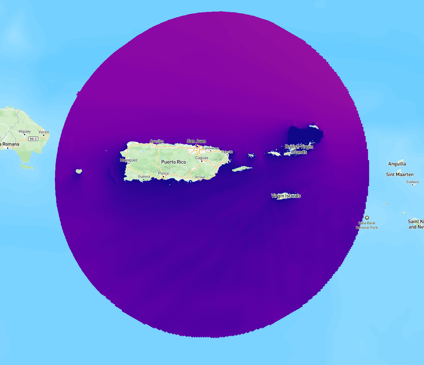
[chicago@ahn2021_us_gulf_of_mexico]
Part of the Gulf of America dataset, using the same grid, variables, and archive period.
Gulf of America
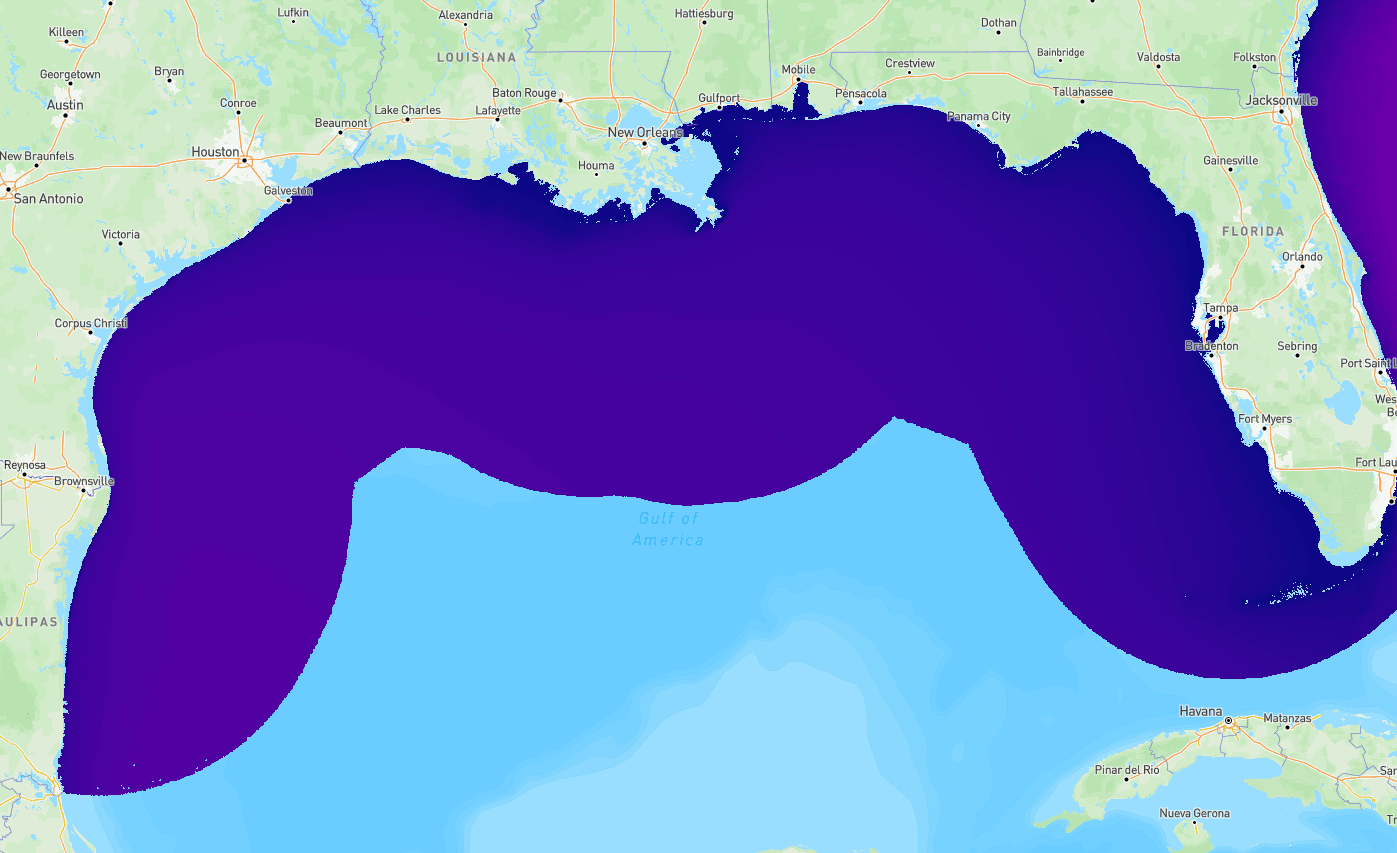
[chicago@ahn2021_us_gulf_of_mexico]
- Grid points: 4,656,637
- File size: ~572.8 GB per year
- Period: 1979–2020 · 42 annual files
- Total archive: ~23.5 TB
- Version:
v1.0.1
Variable definitions (11)
| Variable | Description | IEC Name | SWAN name | Units |
|---|---|---|---|---|
direction_of_maximum_directionally_resolved_wave_power |
Direction of maximum directionally resolved wave power (nautical convention) | \(\theta_{J}\) | degr | |
directionality_coefficient |
Directionality coefficient | \(d\) | ||
energy_period |
Energy period | \(T_{e}\), \(T_{-10}\) | TMM10 | s |
mean_absolute_period |
Mean absolute wave period - equivalent to T_m01 | PER | s | |
mean_wave_direction |
Mean wave direction (nautical convention) | DIR | degr | |
mean_zero-crossing_period |
Mean absolute zero-crossing period | \(T_{z}\), \(T_{02}\) | TM02 | s |
omnidirectional_wave_power |
Omnidirectional wave power | \(J\) | W/m | |
peak_period |
Relative peak period of the variance density spectrum | \(T_{p}\) | RTP | s |
peak_wave_direction |
Peak wave direction (nautical convention) | PDIR | degr | |
significant_wave_height |
Significant wave height | \(H_{m0}\) | HSIGN | m |
spectral_width |
Spectral width | \(\epsilon_{0}\) |
Variable schema (11)
| Variable | Units | Dimensions | Type |
|---|---|---|---|
direction_of_maximum_directionally_resolved_wave_power |
degr | 2,928 × 4,656,637 | float32 |
directionality_coefficient |
2,928 × 4,656,637 | float32 |
|
energy_period |
s | 2,928 × 4,656,637 | float32 |
mean_absolute_period |
s | 2,928 × 4,656,637 | float32 |
mean_wave_direction |
degr | 2,928 × 4,656,637 | float32 |
mean_zero-crossing_period |
s | 2,928 × 4,656,637 | float32 |
omnidirectional_wave_power |
W/m | 2,928 × 4,656,637 | float32 |
peak_period |
s | 2,928 × 4,656,637 | float32 |
peak_wave_direction |
degr | 2,928 × 4,656,637 | float32 |
significant_wave_height |
m | 2,928 × 4,656,637 | float32 |
spectral_width |
2,928 × 4,656,637 | float32 |
Metadata (6 fields)
| Field | Type |
|---|---|
latitude |
float32 |
longitude |
float32 |
timezone |
int16 |
depth |
float32 |
distance_to_shore |
float32 |
jurisdiction |
str[19] |
Limitations
Important Limitations
- Hindcast, not measurements. Model output does not replace in-situ buoy observations.
- Not design-grade by itself. Class 3 assessments require site-specific measurements and validated local modeling.
- Skill varies by region. Validation was performed against NOAA buoys for selected sites; accuracy is generally higher offshore and lower in complex nearshore areas, near domain boundaries, and ice-affected regions (Alaska).
Data Access
Wave energy resource characterization data is available in three data products that serve different needs. Start with the Atlas for visual exploration, then move to the API or raw files as your analysis deepens.
| Use Case | Data Product | Reference |
|---|---|---|
| Explore the resource spatially, compare regions | Marine Energy Atlas | Atlas guide |
| Download time series for up to ~100 sites | us-marine-energy-resource-python or MHKiT wave.io.hindcast |
Getting Started |
| Download or slice the full archive | HSDS or AWS S3 | HSDS Setup · AWS S3 |
| Look up variable definitions and units | Variable reference | Wave Variables |
Start at the Marine Energy Atlas
- Marine Energy Atlas: zero setup, browser-only. Best for stakeholders, initial site screening, and non-programmers.
- MHKiT: 5-line Python queries for point or multi-site time series. Best for feasibility studies and comparing candidate sites.
- HSDS / S3 raw files: direct HDF5 access. Best for bulk extraction, many sites, large regional studies, and reproducible pipelines. Annual files range from ~87 GB (West Coast) to ~600 GB (Gulf of America and Puerto Rico); the full archive is TB-scale.
Site Analysis Example: PacWave South
The visualizations below walk through a Class 2 feasibility workflow at a single grid point near the PacWave wave energy test site off Newport, Oregon (44.62°N, 124.28°W), a U.S. DOE-funded open-water test facility on the West Coast.
What this example covers:
- Pulling a multi-year site time series with MHKiT
- Seasonal and inter-annual variability of key resource parameters
- Monthly wave climate summaries
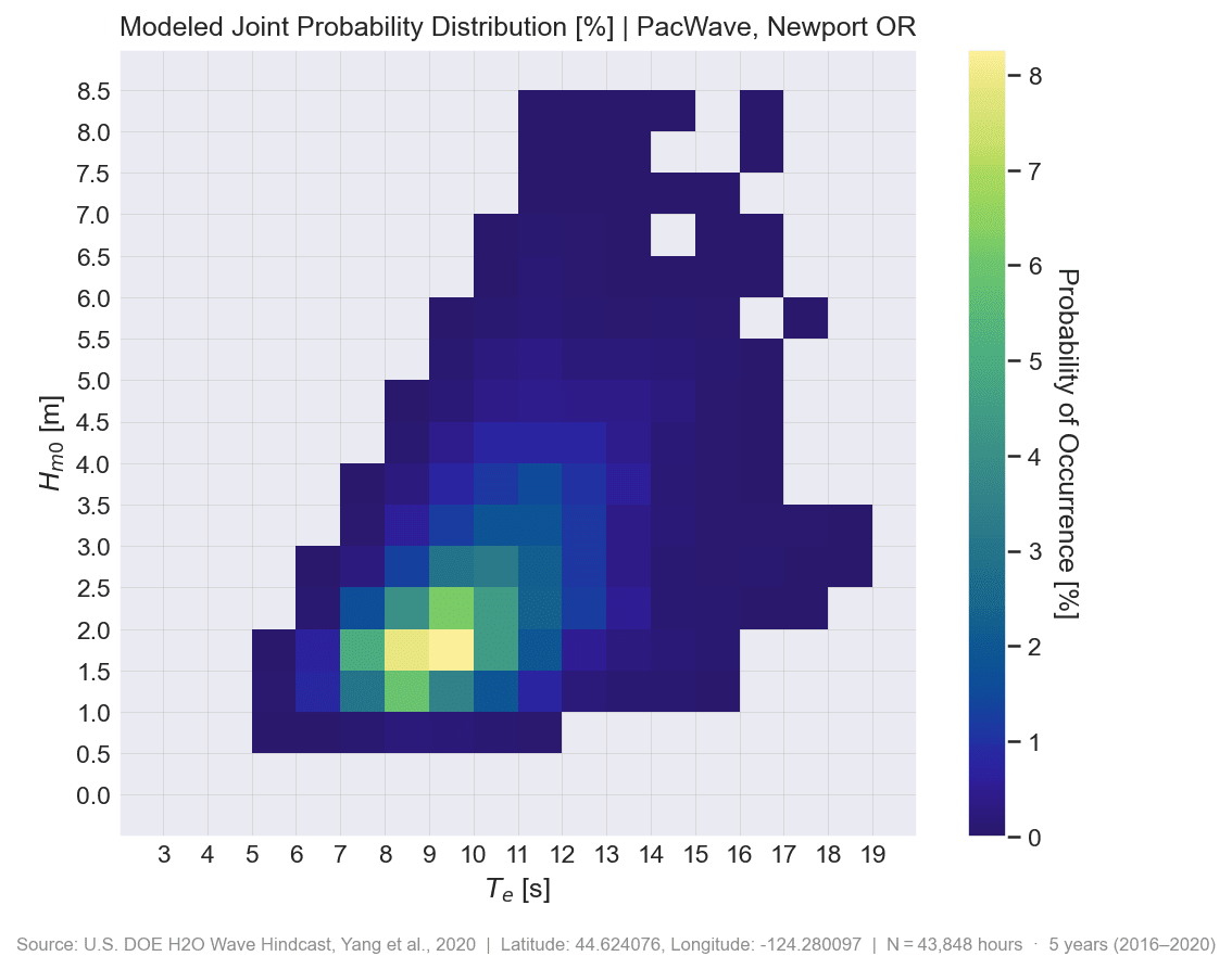
- A wave scatter diagram (\(H_{m0}\) × \(T_e\) joint probability)
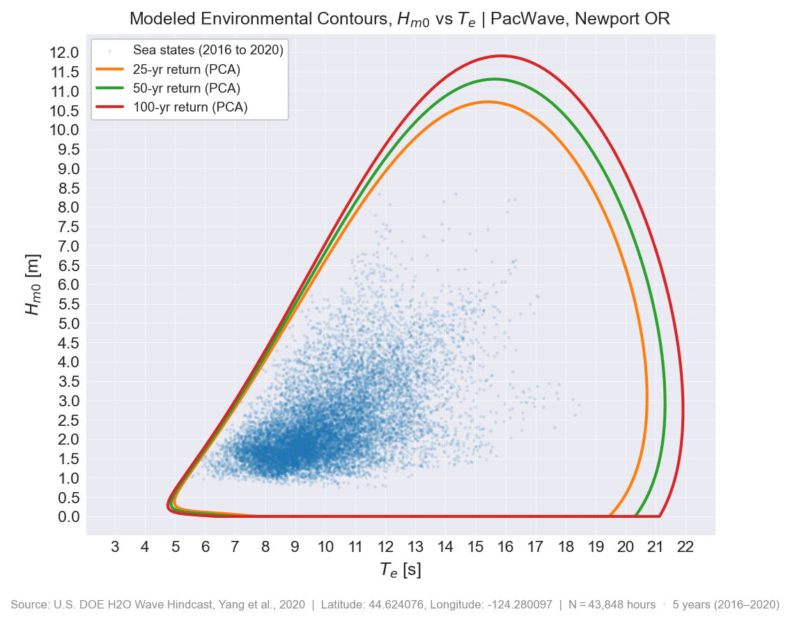
- Environmental contours for extreme sea-state design inputs (25, 50, and 100-year return periods)
Wave Conditions Time Series
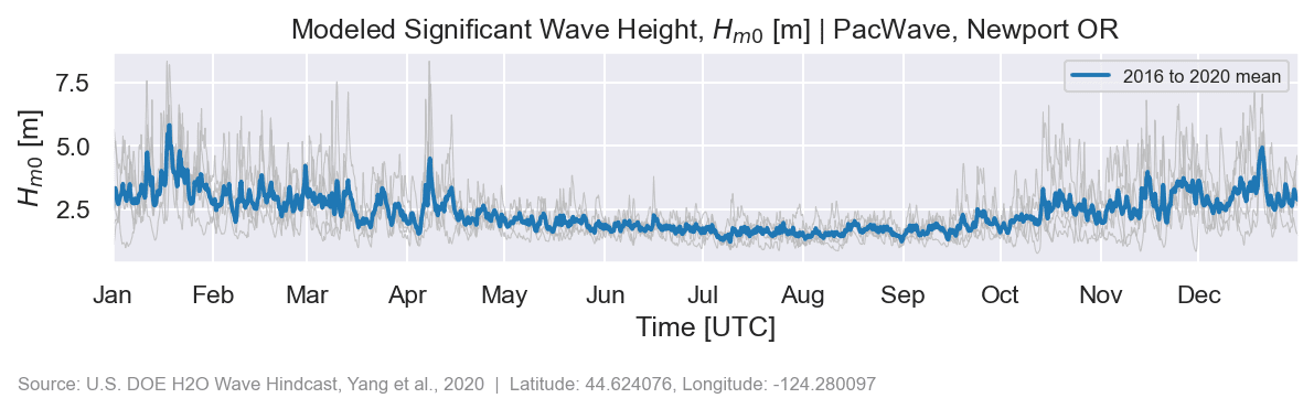
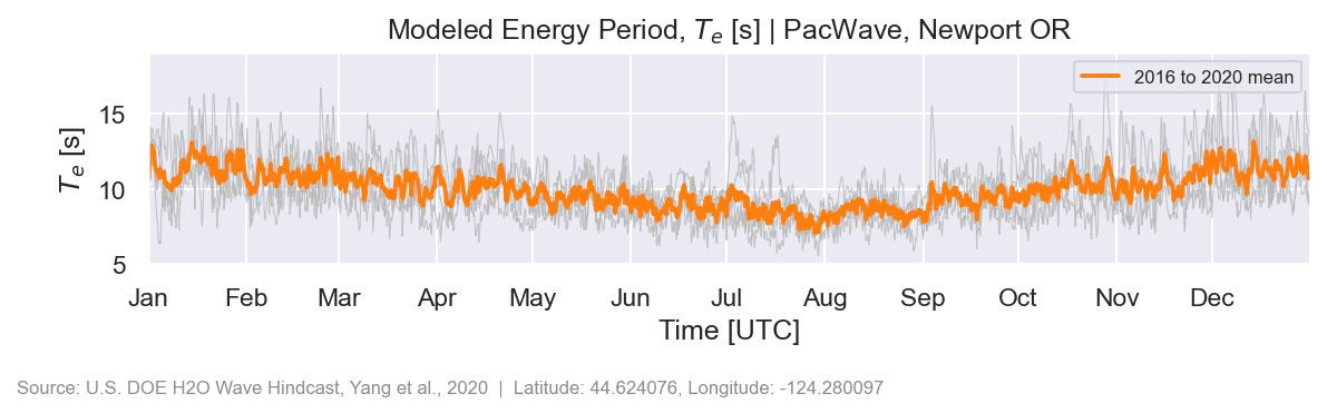
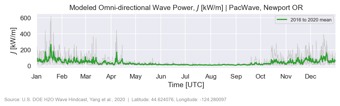
The three plots below show 3-hour hindcast time series at PacWave for 2016 to 2020. Each year is drawn as a grey trace and the 5-year mean is shown in color. Variables are plotted separately so seasonal patterns are easy to read.
Show Python code
def _to_ref_year(s: pd.Series, year: int) -> pd.Series:
    """Map one calendar year's data onto REF_YEAR for overlay alignment."""
    mask = s.index.year == year
    sub  = s[mask].copy()
    new_idx = sub.index.map(lambda t: t.replace(year=REF_YEAR))
    return pd.Series(sub.values, index=new_idx, name=str(year))


def _multiyear_df(s: pd.Series) -> pd.DataFrame:
    """Return a DataFrame with one column per year, index aligned to REF_YEAR."""
    frames = {yr: _to_ref_year(s, yr) for yr in YEARS}
    return pd.DataFrame(frames)


def _apply_ts_xaxis(ax: plt.Axes, index: pd.DatetimeIndex) -> None:
    """Monthly ticks (Jan to Dec labels only; year suppressed for overlay plots)."""
    ax.xaxis.set_major_locator(mdates.MonthLocator())
    ax.xaxis.set_major_formatter(mdates.DateFormatter("%b"))
    ax.set_xlim(index[0], index[-1])
    ax.margins(x=0)
    ax.set_xlabel("Time [UTC]")

def fig_wave_height_timeseries(Hm0: pd.Series, force: bool = False) -> None:
    out = FIGURES["wave_height_timeseries"]
    if out.exists() and not force:
        print(f"  skip (exists): {out.name}")
        return

    df  = _multiyear_df(Hm0)
    fig, ax = plt.subplots(figsize=FIGSIZE_TS)
    _plot_multiyear(ax, df, COLOR_HM0)
    _apply_ts_xaxis(ax, df.index)
    ax.set_ylabel("$H_{m0}$ [m]")
    ax.set_title(f"{TITLE_PREFIX}Significant Wave Height, $H_{{m0}}$ [m] | {LOCATION_NAME}")
    fig.tight_layout()
    _savefig(fig, out)

def fig_energy_period_timeseries(Te: pd.Series, force: bool = False) -> None:
    out = FIGURES["energy_period_timeseries"]
    if out.exists() and not force:
        print(f"  skip (exists): {out.name}")
        return

    df  = _multiyear_df(Te)
    fig, ax = plt.subplots(figsize=FIGSIZE_TS)
    _plot_multiyear(ax, df, COLOR_TE)
    _apply_ts_xaxis(ax, df.index)
    ax.set_ylabel("$T_e$ [s]")
    ax.set_title(f"{TITLE_PREFIX}Energy Period, $T_e$ [s] | {LOCATION_NAME}")
    fig.tight_layout()
    _savefig(fig, out)

def fig_wave_power_timeseries(J: pd.Series, force: bool = False) -> None:
    out = FIGURES["wave_power_timeseries"]
    if out.exists() and not force:
        print(f"  skip (exists): {out.name}")
        return

    J_kW = J / 1000.0
    df   = _multiyear_df(J_kW)
    fig, ax = plt.subplots(figsize=FIGSIZE_TS)
    _plot_multiyear(ax, df, COLOR_J)
    _apply_ts_xaxis(ax, df.index)
    ax.set_ylabel("$J$ [kW/m]")
    ax.set_title(f"{TITLE_PREFIX}Omni-directional Wave Power, $J$ [kW/m] | {LOCATION_NAME}")
    fig.tight_layout()
    _savefig(fig, out)
Monthly Wave Climate
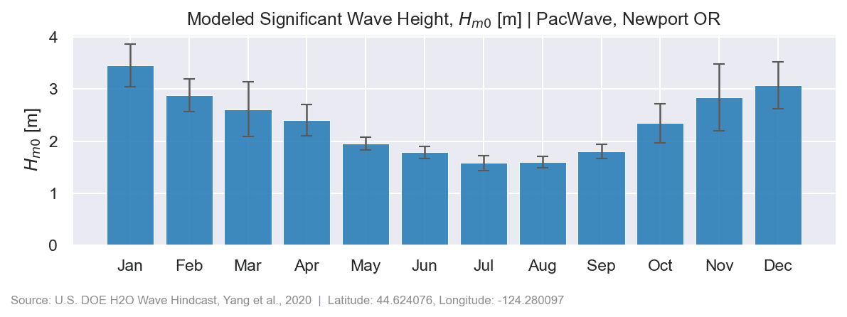
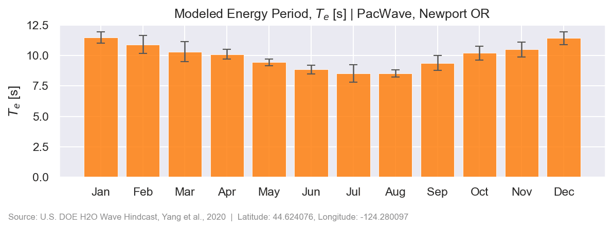
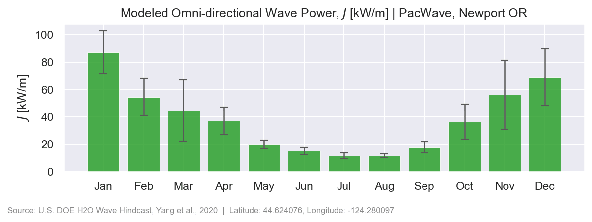
The bar charts below show the monthly mean and inter-annual spread (error bars = ±1 std across years) for each wave parameter at PacWave, capturing the strong Pacific Northwest seasonal signal.
Show Python code
def fig_monthly_barchart_hm0(Hm0: pd.Series, force: bool = False) -> None:
    out = FIGURES["monthly_barchart_hm0"]
    if out.exists() and not force:
        print(f"  skip (exists): {out.name}")
        return
    fig, ax = plt.subplots(figsize=FIGSIZE_BAR)
    _monthly_bar(ax, Hm0, COLOR_HM0,
                 ylabel="$H_{m0}$ [m]",
                 title=f"{TITLE_PREFIX}Significant Wave Height, $H_{{m0}}$ [m] | {LOCATION_NAME}")
    fig.tight_layout()
    _savefig(fig, out)


def fig_monthly_barchart_te(Te: pd.Series, force: bool = False) -> None:
    out = FIGURES["monthly_barchart_te"]
    if out.exists() and not force:
        print(f"  skip (exists): {out.name}")
        return
    fig, ax = plt.subplots(figsize=FIGSIZE_BAR)
    _monthly_bar(ax, Te, COLOR_TE,
                 ylabel="$T_e$ [s]",
                 title=f"{TITLE_PREFIX}Energy Period, $T_e$ [s] | {LOCATION_NAME}")
    fig.tight_layout()
    _savefig(fig, out)


def fig_monthly_barchart_j(J: pd.Series, force: bool = False) -> None:
    out = FIGURES["monthly_barchart_j"]
    if out.exists() and not force:
        print(f"  skip (exists): {out.name}")
        return
    J_kW = J / 1000.0
    fig, ax = plt.subplots(figsize=FIGSIZE_BAR)
    _monthly_bar(ax, J_kW, COLOR_J,
                 ylabel="$J$ [kW/m]",
                 title=f"{TITLE_PREFIX}Omni-directional Wave Power, $J$ [kW/m] | {LOCATION_NAME}")
    fig.tight_layout()
    _savefig(fig, out)
Resource Matrix and Environmental Contours
The joint probability distribution (JPD) maps how often each \(H_{m0}\) and \(T_e\) combination occurs, binned at \(0.5\,\text{m} \times 1\,\text{s}\). The environmental contours (PCA method) define the extreme sea state envelope at 25, 50, and 100-year return periods, providing design load inputs per IEC 62600-101 [@iec_62600_101].
Show Python code
def fig_scatter_diagram(Hm0: pd.Series, Te: pd.Series, force: bool = False) -> None:
    out = FIGURES["scatter_diagram"]
    if out.exists() and not force:
        print(f"  skip (exists): {out.name}")
        return

    Hm0_edges, Te_edges = _wave_bin_edges(Hm0, Te)

    # Bin using left edges as labels so the matrix index/columns are the bin edges
    H_bins = pd.cut(Hm0, bins=Hm0_edges, labels=Hm0_edges[:-1])
    T_bins = pd.cut(Te,  bins=Te_edges,  labels=Te_edges[:-1])

    matrix = pd.crosstab(H_bins, T_bins).replace(0, np.nan)
    matrix = (matrix / matrix.sum().sum() * 100)   # convert counts to %
    matrix.index   = matrix.index.astype(float)
    matrix.columns = matrix.columns.astype(float)

    # Re-index to the full grid so pcolormesh sees every bin slot
    matrix = matrix.reindex(index=Hm0_edges[:-1], columns=Te_edges[:-1])
    Z = matrix.values   # shape: (n_Hm0_bins, n_Te_bins)

    n_hours = int(len(Hm0) * 3)
    fig, ax = plt.subplots(figsize=FIGSIZE_SQUARE)

    cmap = cmocean.cm.haline
    pcm  = ax.pcolormesh(Te_edges, Hm0_edges, Z, cmap=cmap, vmin=0)

    cbar = fig.colorbar(pcm, ax=ax)
    cbar.set_label("Probability of Occurrence [%]", rotation=270, labelpad=16)

    _apply_matrix_axes(ax, Hm0_edges, Te_edges, grid_color="0.80")
    ax.set_title(f"{TITLE_PREFIX}Joint Probability Distribution [%] | {LOCATION_NAME}")
    fig.tight_layout()
    _savefig(fig, out,
             f"N\u2009=\u2009{n_hours:,} hours  ·  {len(YEARS)} years "
             f"({YEARS[0]}\u2013{YEARS[-1]})")

def fig_environmental_contour(Hm0: pd.Series, Te: pd.Series, force: bool = False) -> None:
    out = FIGURES["environmental_contour"]
    if out.exists() and not force:
        print(f"  skip (exists): {out.name}")
        return

    sea_state_duration = 3 * 3600
    n_hours = int(len(Hm0) * 3)

    # Pre-compute all contours so we can size the axes to contain them fully
    contour_specs = [(25, COLOR_C25, "-"), (50, COLOR_C50, "-"), (100, COLOR_C100, "-")]
    contours = []
    for rp, color, ls in contour_specs:
        c = environmental_contours(
            Hm0.values, Te.values,
            sea_state_duration=sea_state_duration,
            return_period=rp,
            method="PCA",
        )
        contours.append((rp, color, ls, np.array(c["PCA_x1"]), np.array(c["PCA_x2"])))

    # Expand bin edges so the largest contour envelope is fully inside the axes
    Te_max_c  = max(Te_c.max()  for _, _, _, _,     Te_c  in contours)
    Hm0_max_c = max(Hm0_c.max() for _, _, _, Hm0_c, _     in contours)
    Hm0_edges, Te_edges = _wave_bin_edges(
        Hm0, Te,
        Te_max_override=Te_max_c,
        Hm0_max_override=Hm0_max_c,
    )

    fig, ax = plt.subplots(figsize=FIGSIZE_SQUARE)

    # Scatter dots: sns palette[0] with opacity
    ax.scatter(Te.values, Hm0.values, s=2, alpha=0.10, color=COLOR_HM0,
               label=f"Sea states ({YEARS[0]} to {YEARS[-1]})", zorder=1)

    for rp, color, ls, Hm0_c, Te_c in contours:
        # Close the contour without re-sorting (sorting scrambles the closed-loop
        # point order into a zigzag that renders as a filled polygon)
        ax.plot(np.append(Te_c, Te_c[0]), np.append(Hm0_c, Hm0_c[0]),
                color=color, linewidth=2, linestyle=ls,
                label=f"{rp}-yr return (PCA)", zorder=3)

    _apply_matrix_axes(ax, Hm0_edges, Te_edges, grid_color="white")
    ax.set_title(f"{TITLE_PREFIX}Environmental Contours, $H_{{m0}}$ vs $T_e$ | {LOCATION_NAME}")
    leg = ax.legend(fontsize=9)
    leg.get_frame().set_facecolor("white")
    leg.get_frame().set_alpha(1.0)
    fig.tight_layout()
    _savefig(fig, out,
             f"N\u2009=\u2009{n_hours:,} hours  ·  {len(YEARS)} years "
             f"({YEARS[0]}\u2013{YEARS[-1]})")
Resource Characterization (IEC/TS 62600-101)
IEC/TS 62600-101 [@iec_62600_101] defines three levels of wave resource assessment, which can be thought of as progressively deeper stages of a development project:
| IEC class | What you are doing | Hindcast supports? | Best access path |
|---|---|---|---|
| Class 1: Reconnaissance | Screening regions, comparing broad areas, identifying candidate sites | Yes | Marine Energy Atlas |
| Class 2: Feasibility | Site time series, seasonal profiles, scatter diagrams, early extreme-value inputs | With caveats | MHKiT or raw H5 |
| Class 3: Design | Device engineering, array layout, certification-grade assessment | Not alone | Site measurements and validated local modeling |
Class 1: Reconnaissance
The Marine Energy Atlas displays time-averaged wave energy resource parameters (significant wave height, wave power, energy period) across all hindcast domains. Grid cells are color-coded by magnitude and a point-query tool returns summary statistics for any selected location.
Class 2: Feasibility
A Class 2 assessment derives site-specific statistics from the full time series. The hindcast provides all six IEC/TS 62600-101 primary resource parameters:
- Significant wave height (\(H_{m0}\)): mean height of the largest one-third of waves
- Energy period (\(T_e\)): spectral period weighted toward low-frequency components; preferred for wave power calculations
- Peak period (\(T_p\)): period at the dominant spectral peak
- Mean zero-crossing period (\(T_z\)): average zero-crossing period derived from spectral moments
- Omni-directional wave power (\(J\)): total wave energy flux from all directions [W/m]
- Directionality coefficient (\(d\)): fraction of wave power arriving from the dominant direction
Point queries can be made using MHKiT:
from mhkit.wave.io.hindcast.hindcast import request_wpto_point_data

# PacWave site near Newport, OR
lat_lon = (44.624076, -124.280097)

# Fetch one year of significant wave height and energy period
Hm0, meta = request_wpto_point_data("3-hour", "significant_wave_height", lat_lon, [2005])
Te,  meta = request_wpto_point_data("3-hour", "energy_period",            lat_lon, [2005])
MHKiT is ideal for up to ~100 sites. For larger studies, switch to HSDS or S3 bulk access:
from rex import ResourceX

wave_file = '/nrel/US_wave/West_Coast/West_Coast_wave_2005.h5'
with ResourceX(wave_file, hsds=True) as f:
    meta       = f.meta
    time_index = f.time_index
    Hm0        = f['significant_wave_height']
    J          = f['omni-directional_wave_power']
Prerequisites
See Getting Started for HSDS/S3 setup.
Next Steps
- Access the data: see Getting Started for HSDS/S3 setup and code examples using us-marine-energy-resource-python, MHKiT, and rex.
- Explore variables: see Wave Variables for full IEC and SWAN definitions of each output parameter.
- Read the references: see References for the publications behind each regional dataset.